OpenCV与AI深度学习 | 实战 | 基于YOLOv9+SAM实现动态目标检测和分割（步骤 + 代码）

本文来源公众号“OpenCV与AI深度学习”，仅用于学术分享，侵权删，干货满满。

原文链接：实战 | 基于YOLOv9+SAM实现动态目标检测和分割（步骤 + 代码）

0 导  读

    本文主要介绍基于YOLOv9+SAM实现动态目标检测和分割，并给出详细步骤和代码。

1 背景介绍

    在本文中，我们使用YOLOv9+SAM在RF100 Construction-Safety-2 数据集上实现自定义对象检测模型。

    这种集成不仅提高了在不同图像中检测和分割对象的准确性和粒度，而且还扩大了应用范围——从增强自动驾驶系统到改进医学成像中的诊断过程。

    通过利用 YOLOv9 的高效检测功能和 SAM 以零样本方式分割对象的能力，这种强大的组合最大限度地减少了对大量再训练或数据注释的需求，使其成为一种多功能且可扩展的解决方案。

2 YOLOv9简介

2.1 YOLOv9简介（You Only Look Once）

YOLOv9性能图示

YOLOv9模型图

    YOLOv9 在实时目标检测方面取得了重大进步，结合了可编程梯度信息 (PGI) 和通用高效层聚合网络 (GELAN)，以提高效率、准确性和适应性，其在 MS COCO 数据集上的性能证明了这一点。

    利用开源社区的协作工作并在 Ultralytics YOLOv5 的基础上构建，YOLOv9 通过信息瓶颈原理和可逆函数解决深度学习中信息丢失的挑战，跨层保留基本数据。

    这些创新策略提高了模型的结构效率，并确保精确的检测能力，而不会影响细节，即使在轻量级模型中也是如此。

    YOLOv9 的架构减少了不必要的参数和计算需求，使其能够在各种模型大小（从紧凑的 YOLOv9-S 到更广泛的 YOLOv9-E）上实现最佳性能，展示了速度和检测精度之间的和谐平衡。

    作为计算机视觉领域的里程碑，YOLOv9不仅建立了新的基准，而且拓宽了人工智能在目标检测和分割方面的应用视野，凸显了该领域战略创新和协作努力的影响。

3 SAM简介

3.1 SAM简介（Segment-Anything-Model）

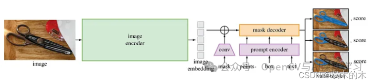
SAM模型图

    分割一切模型 (SAM) 通过简化图像分割来推动计算机视觉向前发展，这对于从科学研究到创造性工作的一系列用途至关重要。

    SAM 利用迄今为止最大的 Segment Anything 1-Billion (SA-1B) 掩模数据集，通过减少对专业知识、强大的计算能力和广泛的数据集标注的依赖来实现分割的民主化。

    在 Apache 2.0 许可证下，SAM 引入了一个基础模型框架，允许通过简单的提示轻松调整任务，反映自然语言处理中的进步。

    通过对超过 10 亿个不同掩模的训练，SAM 理解了物体的广义概念，促进了跨陌生领域的零镜头传输，并增强了其在 AR/VR、创意艺术和科学研究等各个领域的实用性。

    该模型的提示驱动灵活性和广泛的任务适应性标志着分割技术的重大飞跃，将 SAM 定位为研究社区和应用程序开发人员的多功能且易于访问的工具。

4 关于数据集

    该项目利用Roboflow 的RF100施工数据集，特别是Construction-Safety-2子集，来演示集成模型的功能。

https://blog.roboflow.com/roboflow-100/

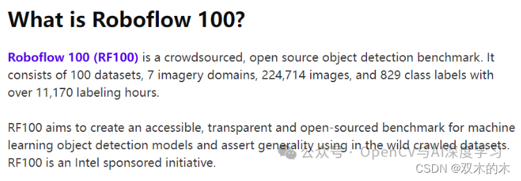
    RF100 是由英特尔发起的一项计划，旨在建立对象检测模型的开源基准。它侧重于 Roboflow Universe 上可用数据集的通用性，提高可访问性并加快人工智能和深度学习的开发过程。

    RF100 构建数据集与 Roboflow 中的其他项目一样，是开源的，可以免费使用。      

5 实现步骤

5.1 实现步骤目录

• 环境设置
• 下载 YOLOv9 和 SAM 的预训练模型权重
• 图像推理
• 可视化和分析
• 获取检测结果
• 使用 SAM 进行分割

  5.2 环境设置

      需要有 Google 帐户才能访问 Google Colab，这是一项免费云服务，为深度学习任务提供必要的计算资源，包括访问高达 16 GB 的 GPU 和 TPU。

      GPU状态检查

      首先，我们确保 GPU 的可用性和就绪性，用于处理和运行 YOLOv9+SAM 模型。

  

  5.3 安装 Google 云盘

      接下来，如果您已经下载了数据集，我们需要导航到存储数据集的文件夹，否则我们可以直接使用 Roboflow 加载数据集。

  from google.colab import drive
  drive.mount('/content/drive')
  or
  %cd {HOME}/
  !pip install -q roboflow
  from roboflow import Roboflow
  rf = Roboflow(api_key="YOUR API KEY")
  project = rf.workspace("roboflow-100").project("construction-safety-gsnvb")
  dataset = project.version(2).download("yolov7")

  5.4 配置 YOLOv9

      数据集准备好后，克隆 YOLOv9 存储库，然后切换到 YOLOv9 目录并安装所需的依赖项，为对象检测和分割任务做好准备。

  !git clone https://github.com/SkalskiP/yolov9.git
  %cd yolov9
  !pip3 install -r requirements.txt -q

  5.5 显示当前目录

      将当前工作目录的路径存储在HOME变量中以供参考。

  import os
  HOME = os.getcwd()
  print(HOME)

  5.6 下载权重模型

      让我们为模型权重创建一个目录，并从 GitHub 上的发布页面下载特定的 YOLOv9 和 GELAN 模型权重，这对于使用预训练参数初始化模型至关重要。

  !mkdir -p {HOME}/weights
  !wget -P {HOME}/weights -q https://github.com/WongKinYiu/yolov9/releases/download/v0.1/yolov9-c.pt
  !wget -P {HOME}/weights -q https://github.com/WongKinYiu/yolov9/releases/download/v0.1/yolov9-e.pt
  !wget -P {HOME}/weights -q https://github.com/WongKinYiu/yolov9/releases/download/v0.1/gelan-c.pt
  !wget -P {HOME}/weights -q https://github.com/WongKinYiu/yolov9/releases/download/v0.1/gelan-e.pt

  5.7 下载图像进行推理

      为了使用 YOLOv9 权重进行推理，我们必须设置一个数据目录并下载一个示例图像进行处理，并在变量中设置该图像的路径SOURCE_IMAGE_PATH。

  !mkdir -p {HOME}/data
  !wget -P {HOME}/data -q /content/drive/MyDrive/data/image9.jpeg
  SOURCE_IMAGE_PATH = f"{HOME}/image9.jpeg"

  5.8 使用自定义数据运行检测

      之后，执行detect.py指定参数对图像进行目标检测，设置置信度阈值并保存检测结果。这将创建一个包含 class_ids、边界框坐标和置信度分数的文本文件，我们稍后将使用它。

  !python detect.py --weights {HOME}/weights/gelan-c.pt --conf 0.1 --source /content/drive/MyDrive/data/image9.jpeg --device 0 --save-txt --save-conf

  5.9 显示检测结果

      然后，我们利用 IPython 的显示和图像功能来展示指定路径图像中检测到的对象，并进行调整以获得最佳观看效果。

  

  5.10 安装 Ultralytics

      安装 Ultralytics 包以访问 YOLO 对象检测模型实现和实用程序，不要忘记导入 YOLO 类以执行对象检测任务。

  !pip install ultralytics 
  from ultralytics import YOLO

  5.11 安装Segment-Anything模型

      现在让我们安装 Segment-Anything 库并下载 SAM 模型的权重文件，为高质量图像分割任务做好准备。

  !pip install 'git+https://github.com/facebookresearch/segment-anything.git'
  !wget https://dl.fbaipublicfiles.com/segment_anything/sam_vit_h_4b8939.pth

  5.12 提取检测结果和置信度分数

      我们需要将 YOLOv9 检测结果保存在上面的文本文件中来提取类 ID、置信度分数和边界框坐标。这里的坐标已经标准化，所以我们先将它们转换为图像比例，然后打印它们进行验证。

  import cv2
  # Specify the path to your image
  image_path = '/content/drive/MyDrive/data/image9.jpeg'
  # Read the image to get its dimensions
  image = cv2.imread(image_path)
  image_height, image_width, _ = image.shape
  detections_path = '/content/yolov9/runs/detect/exp/labels/image9.txt'
  bboxes = []
  class_ids = []
  conf_scores = []
  with open(detections_path, 'r') as file:
      for line in file:
          components = line.split()
          class_id = int(components[0])
          confidence = float(components[5])
          cx, cy, w, h = [float(x) for x in components[1:5]]
          # Convert from normalized [0, 1] to image scale
          cx *= image_width
          cy *= image_height
          w *= image_width
          h *= image_height
          # Convert the center x, y, width, and height to xmin, ymin, xmax, ymax
          xmin = cx - w / 2
          ymin = cy - h / 2
          xmax = cx + w / 2
          ymax = cy + h / 2
          class_ids.append(class_id)
          bboxes.append((xmin, ymin, xmax, ymax))
          conf_scores.append(confidence)
  # Display the results
  for class_id, bbox, conf in zip(class_ids, bboxes, conf_scores):
      print(f'Class ID: {class_id}, Confidence: {conf:.2f}, BBox coordinates: {bbox}')

  5.13 初始化 SAM 以进行图像分割

      使用指定的预训练权重初始化 SAM 后，我们继续从 SAM 模型注册表中选择模型类型以生成分段掩码。

  from segment_anything import sam_model_registry, SamAutomaticMaskGenerator, SamPredictor
  sam_checkpoint = "/content/yolov9/sam_vit_h_4b8939.pth"
  model_type = "vit_h"
  sam = sam_model_registry[model_type](checkpoint=sam_checkpoint)
  predictor = SamPredictor(sam)

  5.14 加载图像进行分割

      通过 OpenCV 库，我们加载图像以使用 SAM 进行处理，为分割做好准备。

  import cv2
  image = cv2.cvtColor(cv2.imread('/content/drive/MyDrive/data/image9.jpeg'), cv2.COLOR_BGR2RGB)
  predictor.set_image(image)

  5.15 结果可视化​​​​​​​

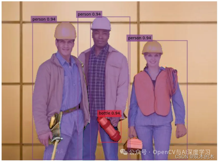
      为了可视化检测和分割结果，我们必须使用 SAM 将边界框转换为分割掩模。我们随机为类 ID 分配唯一的颜色，然后定义用于显示掩码、置信度分数和边界框的辅助函数。coco.yaml 文件用于将 class_ids 映射到类名。

  import matplotlib.patches as patches
  from matplotlib import pyplot as plt
  import numpy as np
  import yaml
  with open('/content/yolov9/data/coco.yaml', 'r') as file:
      coco_data = yaml.safe_load(file)
      class_names = coco_data['names']
  for class_id, bbox, conf in zip(class_ids, bboxes, conf_scores):
      class_name = class_names[class_id]
      # print(f'Class ID: {class_id}, Class Name: {class_name}, BBox coordinates: {bbox}')
  color_map = {}
  for class_id in class_ids:
      color_map[class_id] = np.concatenate([np.random.random(3), np.array([0.6])], axis=0)
  def show_mask(mask, ax, color):
      h, w = mask.shape[-2:]
      mask_image = mask.reshape(h, w, 1) * np.array(color).reshape(1, 1, -1)
      ax.imshow(mask_image)
  def show_box(box, label, conf_score, color, ax):
      x0, y0 = box[0], box[1]
      w, h = box[2] - box[0], box[3] - box[1]
      rect = plt.Rectangle((x0, y0), w, h, edgecolor=color, facecolor='none', lw=2)
      ax.add_patch(rect)
      label_offset = 10
      # Construct the label with the class name and confidence score
      label_text = f'{label} {conf_score:.2f}'
      ax.text(x0, y0 - label_offset, label_text, color='black', fontsize=10, va='top', ha='left',
              bbox=dict(facecolor=color, alpha=0.7, edgecolor='none', boxstyle='square,pad=0.4'))
  plt.figure(figsize=(10, 10))
  ax = plt.gca()
  plt.imshow(image)
  # Display and process each bounding box with the corresponding mask
  for class_id, bbox in zip(class_ids, bboxes):
      class_name = class_names[class_id]
      # print(f'Class ID: {class_id}, Class Name: {class_name}, BBox coordinates: {bbox}')
      color = color_map[class_id]
      input_box = np.array(bbox)
      # Generate the mask for the current bounding box
      masks, _, _ = predictor.predict(
          point_coords=None,
          point_labels=None,
          box=input_box,
          multimask_output=False,
      )
      show_mask(masks[0], ax, color=color)
      show_box(bbox, class_name, conf, color, ax)
  # Show the final plot
  plt.axis('off')
  plt.show()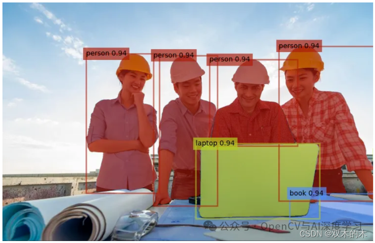

  

  5.16 提取掩码

      最后，我们生成一个合成图像，在白色背景下突出显示检测到的对象，从分割蒙版创建聚合蒙版，并将其应用到将原始图像与白色背景混合以增强可视化

  aggregate_mask = np.zeros(image.shape[:2], dtype=np.uint8)
  # Generate and accumulate masks for all bounding boxes
  for bbox in bboxes:
      input_box = np.array(bbox).reshape(1, 4)
      masks, _, _ = predictor.predict(
          point_coords=None,
          point_labels=None,
          box=input_box,
          multimask_output=False,
      )
      aggregate_mask = np.where(masks[0] > 0.5, 1, aggregate_mask)
  # Convert the aggregate segmentation mask to a binary mask
  binary_mask = np.where(aggregate_mask == 1, 1, 0)
  # Create a white background with the same size as the image
  white_background = np.ones_like(image) * 255
  # Apply the binary mask to the original image
  # Where the binary mask is 0 (background), use white_background; otherwise, use the original image
  new_image = white_background * (1 - binary_mask[..., np.newaxis]) + image * binary_mask[..., np.newaxis]
  # Display the new image with the detections and white background
  plt.figure(figsize=(10, 10))
  plt.imshow(new_image.astype(np.uint8))
  plt.axis('off')
  plt.show()

  ​​​​​​​​​​​​​​

  THE END!

  文章结束，感谢阅读。您的点赞，收藏，评论是我继续更新的动力。大家有推荐的公众号可以评论区留言，共同学习，一起进步。